Data Structures and Algorithms

Time complexity in data structure and algorithms (DSA) refers to the computational complexity that measures the amount of time an algorithm takes to complete as a function of the length of its input. Here are examples of algorithms with constant, linear, logarithmic, and exponential time complexities implemented in Python:

1. Constant Time Complexity (O(1)):

   • Algorithms with constant time complexity execute in the same amount of time regardless of the size of the input data.

   • Example:

def constant_algo(items):
    print(items[0])

# No matter the size of items, this function always prints the first element.

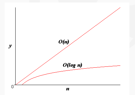
2. Linear Time Complexity (O(n)):

   • Algorithms with linear time complexity have their execution time directly proportional to the size of the input data.

   • Example:

def linear_algo(items):
    for item in items:
        print(item)

# The time taken to print each item increases linearly with the size of items.

3. Logarithmic Time Complexity (O(log n)):

   • Algorithms with logarithmic time complexity typically halve the input data size at each step.

   • Example: Binary search algorithm

def binary_search(arr, target):
    low = 0
    high = len(arr) - 1

    while low <= high:
        mid = (low + high) // 2
        if arr[mid] == target:
            return mid
        elif arr[mid] < target:
            low = mid + 1
        else:
            high = mid - 1

    return -1

# In each iteration, the size of the input (arr) is halved, leading to logarithmic time complexity.

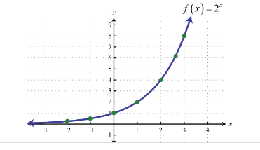
4. Exponential Time Complexity (O(2^n)):

   • Algorithms with exponential time complexity grow very rapidly with the increase in input size.

   • Example: Recursive Fibonacci series calculation

def fibonacci(n):
    if n <= 1:
        return n
    else:
        return fibonacci(n-1) + fibonacci(n-2)

# Each call branches into two more calls, resulting in an exponential growth in time complexity.